“…[samples were] reduced to graphite before AMS 14C analysis at the SUERC AMS Facility.”

To determine the rate of ice sheet retreat it is necessary to determine WHERE the ice sheet margin was WHEN. The WHERE is determined by studying landforms characteristic of glacier margins, such as moraines, erratic boulders, and sediment deposited both onshore and offshore by ice and glacial meltwater near the margins of the ice sheet. The WHEN is determined using different dating techniques depending on the material sampled. For BRITICE-CHRONO we are applying three different dating techniques, (1) optically stimulated luminescence dating (OSL) for sands, (2) radiocarbon dating (¹⁴C) for organic material like shell fragments picked out of sediment cores collected from the sea floor during the research cruises, and (3) surface exposure dating of rock using the terrestrial cosmogenic isotope beryllium-10 (¹⁰Be) in the mineral quartz.

Radiocarbon dating and surface exposure dating rely on being able to measure the abundance of extremely rare radioisotopes in the sample material using a technique called accelerator mass spectrometry (AMS) performed at the Scottish Universities Environmental Research Centre (SUERC) AMS Laboratory. What is extremely rare? Well, the natural abundance of ¹⁴C in modern carbon is 1 part per trillion (10^-12) which gets smaller with the age of the material being dated because ¹⁴C decays after the death of the organism. The ratio between the radioisotope ¹⁰Be and stable beryllium is roughly 10^-13 to 10^-14 for surface exposure dating of BRITICE-CHRONO samples. To put this in perspective, if you counted at one number per second it would take you about 3.25 million years to count to 10¹⁴. In other words, radiocarbon and surface exposure dating is only possible because we are able to count individual radioisotopes among trillions of almost identical stable isotopes.

In scientific papers these  measurements are often summarised in a few words, such as “…[samples were] reduced to graphite before AMS ¹⁴C analysis at the SUERC AMS Facility” or “¹⁰Be/⁹Be ratios were derived from measurements at the SUERC AMS Laboratory”. Neither sentence does justice to the complexity of the method and the efforts of a dedicated team of scientists and technicians. Here I will try to provide some insight into how the concentrations of the extremely low quantities of ¹⁴C are determined using accelerator mass spectrometry (AMS). For ¹⁰Be the process is similar but explaining the differences would add unnecessary complexity in what follows.

Accelerator mass spectrometry (AMS) is an ultra-sensitive technique for isotopic analysis in which atoms extracted from a sample are ionized (the process by which an atom or a molecule acquires a negative or positive charge by gaining or losing electrons to form ions); accelerated to high energies; separated according to their momentum, charge, and energy; and then individually counted after identification as having the correct atomic number and mass. The principle difference between AMS and conventional mass spectrometry (MS) lies in the energies to which the ions are accelerated. In MS the energies are thousands of electron volts (1 keV = 1.6 x 10^-16 J), whereas in AMS they are millions of electron volts (MeV). The practical consequences of having higher energies is that ambiguities in identification of atomic and molecular ions with the same mass are removed.

This is how we make the measurements at SUERC

Fig 1. Cathodes in sample wheel after measurement. The hole in the cathodes contains the sample and is 1mm wide.

Samples come to the AMS Laboratory in the form of pressed cathodes containing a few milligrams of graphite (for radiocarbon) and BeO mixed with Niobium for ¹⁰Be surface exposure dating. It takes a lot of time and effort to get from a sample collected in the field to the cathode stage, but that is another story.

The cathodes are loaded into a 134-position sample wheel together with standard materials that have known isotope ratios.

Fig 2. Sample wheel loaded in ion source.

The wheel is loaded into the ion source, the ion source is closed and pumped down to the same very high vacuum as the remainder of the beam line (steel tube) through which the ions produced in the ion source are going to travel (the correct term is drift, but it does not really convey the speed at which the ions move). We need a very high vacuum (comparable to conditions found in outer space) because we do not want our ions to collide with neutral atoms or molecules drifting anywhere along the 32 metres of beam line.

Fig 3. Section through ionizer

We are now ready to perform some ion sorcery. We heat up a caesium reservoir to generate a Cs vapour in the space between the cathode holding our sample and a heated ionizing surface. Some of the vapour condenses onto the cooled cathode, some is ionised by the ionizer creating Cs⁺ ions that are accelerated and focused towards the sample because the sample cathode is at -5kV compared to the ionizer (Fig 4). The impact of the Cs+ ions on the sample surface causes sputtering of particles from the sample surface.

Fig 4. Cs+ focus lens at front of ioniser (Fig. 3). The sample cathode being ionised is located 1 mm in front of the hole in the lens

Some materials will preferentially sputter negative ions. Other materials will preferentially sputter neutral or positive particles, which pick up electrons as they pass through the condensed caesium layer, producing negative ions. All of this happens within 1 mm of the sample surface. The negative ions are removed from the sample surface and focused into the beam line by an extraction electrode (extractor) set at 15 kV. The extracted ion beam (shown in grey in Fig. 3) is spreading, just like the spreading of light from a torch (which is just another type of particle beam). This is known as beam emittance and it must be kept small to ensure high transmission to the detector. But I am getting way ahead of myself safe to say that we cannot get the emittance of the beam back to the original 1mm diameter at the sample surface and much of the experimental apparatus of the AMS is designed to focus the beam to specific places along the beam line.

Fig 5. Closed ion source. The metal rings around the beam line are part of the 45 kV injector. The apparatus to the left of the rings are for pumping the beam line and and focussing the beam.

So now we have extracted a negative ion beam from our sample material, and the ions are starting to move along the beam line. We accelerate the particles to 66 keV by exposing them to an additional 45kV in the injector (Fig. 5 and Fig 6). The particles pass through a spherical electrostatic analyser (ESA, Fig. 6), where particles with the incorrect energy over charge (E/q) are removed from the beam, before being injected into the accelerator via the injection magnet.

Fig 6. Schematic of SUERC 5MV tandem spectrometer.

The injection magnet separates particles based on momentum (= mass x velocity). For radiocarbon we set the magnetic field to allow particles with mass 14 through the magnet and into the accelerator, but we also need to put carbon-12 and carbon-13 into the accelerator to get the ratio ¹⁴C/¹²C and ¹⁴C/¹³C. Since both ¹²C and ¹³C have lower mass than ¹⁴C we use a magnet bouncing system (MBS; Fig. 6) to give the ion beam more energy so that ¹²C and ¹³C temporarily behave like ¹⁴C. Because ¹²C and ¹³C are much more abundant than ¹⁴C we inject the former two for only a few microseconds per second. While ¹⁴C enters the accelerator we measure the ¹³C current in a low energy Faraday cup and the same is the case for ¹²C when ¹³C is injected (Fig. 6. Inset A). ¹⁴C cannot be measured in a Faraday cup because there are far too few atoms to generate a current.

Unfortunately sample materials are not pure and therefore ion sources do not only produce the ions we want. However the next stage in the process takes care of many of the molecular isobars (= same atomic mass number) such as the hydrocarbons ¹²CH₂^– and ¹³CH^–, which have the same atomic mass number as ¹⁴C and are therefore also injected into the accelerator.

So far the system described is similar to conventional mass spectrometry. The next stage in the ion transport is what sets AMS apart. Up to now the ions have been energised by the ion source and injector to 66keV (the low energy end of the spectrometer), which means they are travelling at roughly 1000 km/s. Next they are accelerated to a speed of roughly 7500 km/s by exposing the negatively charged ions to a 4.5 MV positive charge at the terminal in the centre of the 8 m long accelerator tank (Fig. 6 & 7).

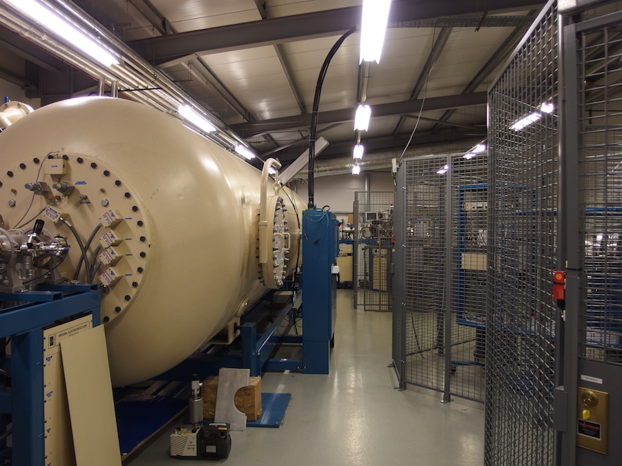
Fig 7. Accelerator pressure vessel known as the tank. It is filled with an insulating gas.

When the negatively charged ions reach the terminal they pass through a gas stripper (Fig. 6). The collisions between the ions and the gas removes electrons from the ions thereby changing them from being negatively charged to being positively charged. The terminal voltage is set to remove at least three electrons because by this process molecular isobars of ¹⁴C (such as ¹²CH₂^– or ¹³CH^–) are destroyed due to the high instability of their positively charged forms, and atomic C⁺ ions such as ¹²C⁺, ¹³C⁺, and ¹⁴C⁺ can be separated due to their different mass to charge ratios. Once the now positive atomic ions emerge from the stripper they find themselves next to a very high positive charge (4.5 MV in the case of radiocarbon) and they accelerate away from this, hence the term tandem accelerator (two acceleration steps). The particles emerge from the tank at a velocity of greater than 17000 km/s (that’s equivalent to traveling around the Earth at the equator in just over 2 seconds), the high-energy part of the AMS.

The particles now enter another mass spectrometer, the analysing magnet (Fig. 6), where the ¹²C⁺, ¹³C⁺, and ¹⁴C⁺ are separated according to momentum. ¹²C⁺ and ¹³C⁺ currents are bent more than ¹⁴C⁺ and are collected and measured in Faraday cups, while ¹⁴C⁺ is allowed to continue on towards the gas ionisation detector. Even after all of this the ion beam still contains ions with incorrect mass, energy, or charge as a result of energy- or charge-changing collisions with system components or residual gas. Unfortunately these interferences mimic the path of the ions of interest. Some of them are removed by another electrostatic analyser (ECA) before the remaining particles arrive at the gas ionisation detector where the final identification and counting of atoms takes place (Fig. 8).

Fig 8. Detector (foreground) and electrostatic analyser (background).

As the ions enter the detector they are slowed down and stopped by passing through a gas. Each atom ionises some of the gas and the resulting electrons are collected, amplified, and digitised. In this way the path and location of each atom arriving in the detector can be determined and each arrival counted. The gas ionisation detector allows us to determine the atom species because heavier atoms travel further and deposit more energy than lighter atoms. This capability allows us to set the electronics to separately count ¹⁴C atoms and different interferences arriving in the detector (Fig 9).

Fig 9. Detector spectrum of one 6 minute measurement. Red dots (n=40933) are counted 14C events. Black dots (n=430) are scattered 14C and Lithium atoms (labelled) that have made it into the detector.

To make all of this possible requires every component of the accelerator mass spectrometer to operate together within very tight tolerances. Even when everything is working well, each time a new sample wheel is introduced into the ion source the conditions inside the ion source vary slightly and the machine has to be very carefully tuned to these new conditions prior to commencing the measurement of the precious samples. Once satisfied the AMS is operating within the necessary limits each sample is measured until measurement statistics are met (usually within 8 measurements), or the sample is exhausted. Each individual measurement lasts about 6 minutes. For high precision measurements it is not unusual to measure a sample for a total of 1 to 1.5 hours. Thus to complete the measurement of a sample wheel is a multi-day undertaking during which the AMS has to be continually monitored for any changes in the condition of multiple machine components that could compromise measurement integrity.

The ¹⁴C/¹³C ratio for each measurement is derived from the counted ¹⁴C atoms in the sample divided by the number of ¹³C atoms calculated from the ¹³C current in the high energy Faraday cup. The final ¹⁴C/¹³C ratio for each sample is the average of the combined ¹⁴C/¹³C ratio measurement for the sample, normalised to known standard materials that were measured in the same wheel. It is this final ¹⁴C/¹³C ratio that is used to calculate the radiocarbon age for the sample.

I hope the above summary provides a little bit of insight into what is meant when you come across sentences like “…AMS ¹⁴C analysis were made at the SUERC AMS Facility” in the literature.

Derek

End of an Era ……….for the mighty British-Irish Ice sheet and our mammoth fieldwork campaign.

By Chris Clark (with photography by Alex Ingle)

Voyages around a former ice sheet…..

After a decade of dreaming and years of planning our team of 40 data-hungry geoscientists were given the scent and released from their cages (~desks) with the audacious task of blitzing the whole ice sheet to find samples for dating its retreat. This started in November 2012 in a grey drizzle at Seisdon sand and gravel quarry near Stourport and finished 09:30am 1st August 2015 in bright sunshine when we extracted our last sample, a seafloor core, from the Cleaver Bank in the southern North Sea. It really has been an epic two and half years witnessing the Terrestrial Team with sun-cream in the Scilly Isles to shivers in Shetland, and with dressing gowns in Donegal to JCBs in Norfolk. We really did covered the ground from south to north and east to west and snuck in 28 – yes 28 – different islands of Britain and Ireland, including Scilly Rock and Foula. When samples were not easy to spot and grab, we used radar, seismics and some occasional guesses to work out where to dig with shovel or digger or to core the hidden sediments. It is not quite true that no stone was left unturned, but I have been amazed at how close we got to that, thanks to some amazing levels of energy and motivation; it is indeed lucky that our team displayed traits of obsessiveness and kleptomania when it came to sampling. Bloody well done to all.

This slideshow requires JavaScript.

So our very last sample (core 179-VC) on BRITICE-CHRONO has now been collected, marking the end of Cruise Two on RRS James Cook. Even though we never got to shout ‘One hundred and …eighty’ it is more than we had planned. We have sailed, steamed, or dieseled 8971.65 kilometres, taking in Skye, Rona, Shetland, and more North Sea banks including (the infamous Dogger) that you could shake a stick at. We have sampled deep (525 m) and very shallow (19 m), and calm and troubled (force 7). Our ship-track might look erratic to some but, as they say in marketing non-speak, it comprises a subtle blend of caution and well-planned targets with a hint of adventure and wild abandon yielding a truly inspiring collection of mud and sand to sate the yearnings of the most inquisitive discerners of ice sheet curios.

The loot under the care of Team Marine (Lou and Margot)

The haul, now sat in our refrigerated lorry-container and packed in plastic tubes was obtained by lowering our vibro- and piston corers through 18,891.4 metres of seawater and extracting over half a kilometre of sediment (Rich says 542.4 m). As well-known, of course, it is not the length that counts, but the quality. It will be some time however before we know which cores, places and transects yield the best shells and forams for dating, but Margot and Lou have already bagged, sifted and labelled the celebrity shells which we think have the best stories to tell….’well there was this bloomin’ huge great wall of ice that kept crashing down, and would you believe what happened next….’.

Science crew of the RRS James Cook cruise JC123

Thanks to Colm and his science team, the Captain and crew and the geological survey coring teams, and the weather, some good planning, crazy hunches and some luck, this scientific cruise has been a great and enjoyable success. We have a mammoth payload that we hope will provide a legacy of new information for decades. It has been a pleasure having Alex, the ever-present black ninja-photographer on-board, – he stalks, clicks and then runs – in his quest to document our highs, lows and silly moments. Hopefully you have already seen much of his work.

This slideshow requires JavaScript.

We set out to do 50 years work in five. Taking this cruise with last year’s, which circumnavigated Ireland, along with our >300 person-days of terrestrial fieldwork we have bagged around 15 tonnes of samples for dating and I hope you agree that we have been around a bit. Sorry if we missed your patch, why don’t you have a go? It is an end of an era for our sampling effort. As project leader, I now breathe a large sigh of relief that it is over and has gone so well, phew and phew again. There is a tinge of sadness though, that we all feel as the fun, bonhomie and making of new friends on hard-won field exploits has now ended. No more pie shops or sneaky pints. Team Terrestrial (Rich and his gang) and Colm’s Marine Crew, can now stand-down to great applause. Derek’s Geochron Team have their work cut out to carefully analyse all the samples and then our Transect Leaders (Tom, Dave, Rich, James, Colm, and Sara) will rise to the challenge of making sense of it all and telling us the story that the shell started to blurt out.

Taking things one day at a time

Chris Clark, signing off on behalf of BRITICE-CHRONO, currently steaming 11 knots, homeward bound, over the Tea Kettle Bank of the southern North Sea. All cores logged and packed and the pinging geophysics finally turned off.

1 o’clock, 2 o’clock, 3 o’clock rock (well…compressed mud), you can rock around the clock….

By Margot Saher and Lou Callard

Take some of the ‘finest’ brains in the country. Put them on a state-of-the-art research vessel which is filled to the brim with geophysical equipment, and has its own core scanning lab. Imagine what one could do with that! And what do we do with it? What is the scientific treasure we hunt? Mud. Six weeks at sea for mud (occasionally sand…)? We’ll be scrutinising it for years to come! Without mud the whole endeavour would be a failure; the mud must be treasured, cared for. It is the sedimentary archive that could answer the question of when and how the British-Irish Ice Sheet vanished. It is the wet lab coring teams that handle, care for and love the mud. There are two shifts: the Night-watch from midnight to noon, and the Day-team from noon to midnight. Whilst in the lab and, more importantly, out on deck, these have to wear armour: PPE (Personnel Protective Equipment) – a hard hat, hobnailed boots and some rather unflattering (generally oversized) overalls. The overalls are optional, but a sensible option at that; the job is a messy one, so unless you have an endless supply of clothes…. As the British Geological Survey (BGS) core team recover the mud to deck we have to wait – impatiently. How much have we recovered, and is it the right stuff? Even before the barrel is laid down we swarm expectantly around its end to get the first glimpse (and touch) of the treasure. The strength of the mud gives us so much information; we prod it, taste it…. Does it feel like silt, sand, clay; is it stiffened, reflecting the weight of former ice sheet bearing down on it? We recover everything from the core shoe, the core catcher; whatever sticks or falls out of the liner gets bagged, labelled, photographed and stored cool. But what is inside the liner is what we really want, it contains the story of the ice coming and going from the waters around these islands.

Heave

Ho

The liners are not easily released from the barrel; muscles are needed to get it out, and a tug-of-war ensues of scientists, BGS engineers, crew, random passers-by, anyone versus the barrel. But once the liner is out, it’s ours. The muds we desire are only useful if we know exactly where they are from, so labelling is everything. Every single core section has its own unique label, which will end up on its liner, caps, wrapping material, and the box it’s stored in. There are yellow caps for the tops and black for the base of each segment; which way is up matters! And that is only the beginning; there is no such thing as over-labelling, and that holds for cores sections, record sheets, scanned records, spreadsheets, photographs……

Lou: “The day shift consists of Steve, Zoe, Catriona, Kevin and me. Whilst Colm and Katrien spend the day planning where we will core next, we collect and process the cores. Generally our day starts at 11:20 with breakfast, which also happens to be lunch for the other crew members. Breakfast can be anything from a curry to fish and chips. Today’s option was Thai fish cakes, with noodles and sweet chilli sauce. Although having such a large meal first thing was rather odd to begin with, six weeks in it seems quite normal and a bowl of cereal would now disappoint. Shift begins with the midday handover meeting and our goodnights to the night team.

This slideshow requires JavaScript.

Then work begins! We spend most of our shift either out on deck collecting and cutting the cores, or in the wet lab splitting, logging and packing the cores away with a constant dual stream of material either from the deep or from the MSCL cave. Frequently we split over 20 sections during our shift, and often it’s more than 25. Each section is 1 m long with each 1 m weighing between 10-12 kg, so after 12 hours of carrying, splitting, logging and packing it is a good workout. So the coring job may seem rather unglamorous and exceptionally mucky, and involves hard manual labour; it is also an exciting and rewarding part of the cruise. The sub-bottom profiles and bathymetry data provides a tantalising look at what might lie beneath, but it is only when the core is taken and the material viewed that you know whether or not we have captured the right material needed for the project, and whether there is something we can use for dating. Sometimes we are disappointed normally if we fail to guess correctly in the ‘guess-the-core-length’ sweepstake (Steve is slightly in the lead at the moment), but when a good core is opened, it changes the mood of everyone involved.

Our work still isn’t quite complete, cleaning and maintaining the lab ready for the night team, labelling, cropping and archiving all photographs, and Zoe dutifully scans all of the deck sheets. At midnight the night team relieves us and then we head either straight to bed or take a detour past the kitchen to get a post shift snack. A day shift favourite is Nutella (somewhere in the multi-verse other nutty spreads might exist) on toast. It is hungry work, coring!”

Margot: “the Nightwatch consists of Kasper, Riccardo, Jenny, myself and occasionally Richard (if he can drag himself away from the Geophysics, picking core sites and mostly chatting on deck). As we start our shift, we tend to find ourselves in the middle of a coring transect that has been planned before, so we of the night often start our shift on station, vibrocoring. We’ve discovered that Riccardo has a special talent for working hard but still staying clean, while Richard has the useful talent for removing almost any sediment from an unwilling core catcher. Kasper’s Danish (or Viking) muscles come in handy for removing the liner from the barrel, and Jenny has useful BGS contacts (which saves us, for instance, from running out of sample bags). I myself have developed the modest knack of writing upside down, for liner labelling purposes.

This slideshow requires JavaScript.

Splitting and description has to wait until we receive cores from Elke and the core scanner cave, and she works 6AM to 6PM. The early part of the shift can be quite calm, if the core stations we have picked are far apart. Quite often nature festoons such a quiet early part of the shift with an amazing sunrise. The pace picks up dramatically as the cores start to emerge from the MSCL cave. It can get a bit hectic if we’re busily splitting and describing, interrupted by receiving new cores from the seabed. Core sections everywhere! But the splitting is exciting, as we get to see the whole sedimentary sequence for the first time. Do we have the ideal core, which consists of a subglacial till at the bottom, conformably overlain by marine sediments deposited after the ice retreated? Are there perhaps some nice shells in it for radiocarbon dating? When we see something we could use for 14C dating, we take it out. As we are coring, we have a competition running: guess the core length. It is very tight at the moment; Riccardo is in the lead, closely followed by Jenny, and Richard is trailing miles behind, but it all can still change, even with only two days to go. Eventually noon arrives, when we hand over to the day team, and then plonk down tiredly for lunch, which, for us, is more like late supper. After lunch and a cup of tea it’s bedtime! And then at around 11PM (ish) we get up again, and the sequence repeats.”

Treasure…..

As we both write this, the 212th core has been recovered from the large moraine in outer Galway Bay. There is some 6 tonnes of mostly mud in our refrigerated container, and we have picked more than 100 shells for dating. But we know exactly where every kilo came from, what it looks like, and which ones we want to target for further research. When we get back on land, we can hit the ground running…..

Photography mostly by Alex Ingle, except where it isn’t….

An Engineers Apprentice

By Claire Mellett and Jenny Gales (British Geological Survey)

A typical day for us usually involves sitting behind a desk staring at a computer in the basement of the BGS Edinburgh office. As marine geologists we are tasked with mapping the seabed and sub-seabed for government and commercial interests. Fundamental to this is an understanding of how geological processes such as ice, rivers, wind, waves and tides have shaped the seabed over long periods of time. Our field area is inaccessible to us as it is drowned beneath sometimes thousands of metres of water and we rely on remote sensing data such as bathymetry and seismic to image the seafloor and make our interpretations. Once we have “guestimated” geological conditions we need to prove them with physical samples and this is where the BGS Marine Operations team comes in.

When carrying out our own research we focus on finding the most suitable site that will provide an answer to whatever question we are asking and we don’t spend too much time thinking about how the sample is recovered. Luckily we have a BGS Marine Operations team comprising electrical, mechanical and design engineers that can build and adapt equipment to meet our expectations. However, ignorance isn’t always bliss and by understanding how different rigs work and the logistics involved in transporting, fitting and fixing equipment on different vessels all around the world, we will have knowledge of how our data was collected and the limitations of its use. Claire: “I thought I would be fairly useless as a member of the operations team given that I am a typical “pen pusher” but I went in with an open mind willing to try anything. As the weeks have gone by I find it easier to lift the barrels meaning I must be getting stronger. I also seem to have started a scrap metal collection as I keep finding bolts and washers in all my pockets. This apparently proves your worth an engineer (according to Garry, one of the BGS engineers)”.

This slideshow requires JavaScript.

After a while we decided to formalise our training so made ourselves engineer’s apprentices. As part of the apprenticeship we came up with list of skills that needed to be developed. These include tasks like winch operation (which is the most stressful part of the apprenticeship), vibrocore assembly, vessel awareness (Claire: “I can now distinguish the bulkhead from the deckhead”), health and safety and vibrocore driving. This last skill is obviously very important as when carrying out this task you get the comfiest seat in the container right next to the heater (which also reclines for when you’re on night shift). Additional skills every seafaring apprentice must have include coffee and tea making (including biscuit acquisition) to keep the team going on twelve hour shifts, rope skills (Jenny: “we can now both tie a rolling hitch with two half hitches to get the core liner out of the barrel”) and radio etiquette which varies greatly depending on accents. The final part of the training is tool recognition. We are getting good at this although there appears to be a nomenclature issue depending what tradesman you get e.g. a “toffee hammer” is apparently the same as a “quarter pound ball pein hammer”.

This slideshow requires JavaScript.

We do have it easy in comparison to the rest of the BGS engineering team as when things break down, which is likely to happen when you’re at sea for a long time, they surprise us by just fixing things. As engineers, this is their job, but it still gets us each time they make something work. For example, we are running low on core catchers as the geology keeps destroying them so we decided to just make some. A bit of improvisation and some welding and we have a new supply of core catchers, voilà!

The work day for an engineer’s apprentice is so refreshing yet tiring. We are outside all day which is delightful when the sun (or moon) is reflecting off a reasonable calm sea with big white fluffy clouds on the horizon. Even when the rain is horizontal and the waves are crashing over the deck, we still look forward to getting out to work. When compared to the often solitary life of a scientist where you exist in your ideas, it is a welcome change to be working outside as part of a team of engineers and ship’s crew physically collecting the scientific data you spend most our time working on. Claire: “I must add here that the ship’s crew on board are all extremely patient with helping us in our training (especially when it comes to winch operation!)”.

We keep being asked if we prefer being a scientist or part of the operations team on a research cruise and it’s a difficult question to answer. Claire: “It is a bit of a holiday for me being an engineer’s apprentice as it is not my profession, therefore all the pressure is on our trainers (Iain and Mike’s) shoulders. I do appear to spend a large part of the day laughing (usually at myself) which is a sign I am enjoying the work. However, if I had a 90 m research vessel at my disposal, as a scientist, I can only imagine the fun I would have!”.

(Selected photography by Alex Ingle)

A room without a view……

By Elke Hanenkamp (MSCL Operator)

Enter my lair

Six o’clock in the morning on board the RRS James Cook somewhere on the edge of Malin Sea in 1500m of water, and my shift as the MSCL operator starts right now. The dayshift (midday to midnight) is still fast asleep and the nightshift (midnight to midday) scientists are eagerly (or maybe more fatalistically) awaiting my arrival. The beginning of my shift marks the start for them that cores can finally be split and described soon (meaning more work for them), therefore I have been jokingly nicknamed “the harbinger of cores”.

My role during this expedition is to collect physical properties data (density, porosity etc) from the vibro and piston cores before they are split on board. I am operating a Geotek Multi-Sensor Core Logger (MSCL) in a containerised lab (also known as “the container cave”, I am in there all the time holed up with the cores). So the obvious question is – what is happening behind the closed door of the container? After the cores come aboard, they are cut into sections and labelled, and then stored for at least 6 hours inside the container to equilibrate to ambient temperature. Only after this period, the cores will be measured on the MSCL, because some of the sensors are temperature sensitive. It is not possible to prop the door open during the measurements, fluctuations in temperature would influence the data. That’s why I am holed up in the container most of the time, every so often delivering already measured cores to the scientists for splitting or taking newly labelled cores into the container.

The Multi Sensor Core Logger is a quite versatile core measurement system, equipped with four sensors – Gamma Density, P-Wave Velocity, Non-Contact Resistivity and Magnetic Susceptibility. While the core is pushed past the stationary sensors, it is scanned, and data from all four sensors is collected at once when the core pauses at a measurement point (in this case every 2 cm). Sequential core sections are loaded on to the logger, this way a complete core can be logged in a continuous process while the data is displayed graphically in real time on the computer. Typically, with measurements being done every 2 cm, a 1 m section can be logged within 15 min, but overall measurement time for one whole core depends on the amount and length of each individual section the core is cut into earlier. The shortest core section we had so far measured only 21 cm. The amount of cores sections measured each day highly varies, but a couple of days ago, 45 sections were measured on the MSCL within my 12 hour-shift, with a total length of a little bit over 41 m (a new record).

This slideshow requires JavaScript.

The MSCL gives us a non-destructive way of analysing cores before they are split and sampled. The measurements can help to characterise the physical nature of the individual cores, e.g. lithology, density, porosity, and will be used in combination with core descriptions and various geochronological data to better understand the timing of ice sheet recession. The high-resolution dataset from the MSCL should also allow us to make correlations between individual core sites in the Celtic, Irish and Malin Seas fringing the North Atlantic.

A view of the world

BRITICECHRONO Fieldwork on the Isle of Man ~ November 2013

The leaving of Heysham is nothing like the leaving of Liverpool

By Richard Chiverrell

For Transect 3 of BRITICECHRONO, THE Irish Sea East, north from the terrestrial component in Shropshire-Lancashire, much of the remainder will be be dealt with during the marine cruises. The Isle of Man is the clear exception with excellent terrestrial exposure of the Quaternary geology; it is an excellent candidate region for dating the decline of the ISIS. The Isle of Man occupies a position astride successive ice advances through the Irish Sea Basin and records evidence of fluctuations of ice in the Irish Sea basin. The glacial geology of the Isle of Man is extremely well known, and this knowledge forms the basis for recent BRITICECHRONO fieldwork on the Isle of Man.

Geomorphology of the Isle of Man (Thomas et al., 2006)

Team Isle of Man consisted of Richard Chiverrell, Matt Burke, Daniel Schillereff (all Liverpool University), and David Roberts (Durham University), with meticulous planning (and no hastily rearranged flights) the intrepid team took off for autumnal bedock, erratics, sands, Manx queenies, cliff sections, gravels, sands, buried soils (?), kettlehole basins and ground penetrating radar on 4^th to 9^th November 2013….. We divided the Island five sectors documenting the northwards retreat, a) the Plains of Malew and adjacent hills (the South); b) the Peel embayment (the Central Valley) and on the northern plain c) outwash deposits of the Shellag Formation (the initial retreat); d) ice marginal sandar deposits associated with the Orrisdale Formation ice marginal oscillations (previously dated by Ian Thrasher) and e) outwash deposits of the Jurby Formations lain down during a more substantial 2-3km readvance. Together geochronology from these sectors would document the phased retreat across the Isle of Man and secure the timing of two well defined readvance episodes (Orrisdale and Jurby events).

Day 1 Monday – Travel and reccie day for some: Roberts, Dave, was first to arrive, apparently having set off before dawn, from whence he set gainfully on reacquainting himself with some former haunts, having spent a happy 12 months on the Island as a post doc in the mid- to late 1990’s. A very good day followed, bedrock sites on the southern flanks of Man, and a search for the famous Foxdale erratic train….. Meanwhile following a 9am lecture to the second years on European peat climate records, Chiverrell (Rich) tried to find his unusually elusive postdoc, Burke (Matt) who had been set the not insignificant challenge of cramming too much equipment into a car that had now seen better days. But second success of the day followed, 2x GPR antennae, 1x RTK Trimble GPS, tripods and staffs, monolith tins, 3x gamma detectors, the Roberts Rocksaw and cosmo kit, luminescence tubes and gearing, plus two scientists, can fit….  Third success, catching the boat from Heysham to Douglas, only 60 mins early for check in this time….. By 10.30 we had all collected in Andreas in the far north of the Islands, via in Dave’s case some old haunts in Douglas and a fine meal in the Sulby Glen Hotel for Matt and Rich.

Day 2 Tuesday – The Plain of Malew: The excellent recognisance by Dave helped us make short work of the very south of the Island. Bedrock samples a quartz arenite and quartz vein (sample 1 and 2) from Cregneash Peninsula overlooking the Calf of Man, where ice skirting the western flank of the Island has scoured and streamlined the topography and permission given by a very helpful landowner. The search for outwash sand and gravels for OSL proved slightly more taxing, with in the late afternoon a former bedrock quarry near Ronaldsway airport, Turkeyland Quarry, yielding a thin outwash deposit (sample 3) and a very enigmatic buried weathered soil, possible 14C target. And a fine dinner of Manx queenies and skate courtesy of chefs Matt and Dave. The final member, Schillereff (Dan), of the team flew in that evening to provide expertise on the kettlehole sediments, and revisit what might have been the locale for his undergraduate dissertation.

This slideshow requires JavaScript.

Day 3 Wednesday – The Foxdale Granites and moving northwards:With permission from Manx National Heritage (Isle of Man Government) in order, the ‘holy grail’ site for BriticeChrono was very quickly lined up, the Foxdale granites. Ice flowing north to south penetrated through valleys from Glen Maye and Foxdale valley building to eventually bury and consume the Isle of Man. In Foxdale at the col at the head of the valley (~200m) a granitoid is exposed, and the erratic train holds a place of significance in the geological literature, including the attention of Charles Darwin (1842) as a classic example of transport of glacial boulders from low to higher ground including the summit of South Barrule. With the permission and assistance of Manx National Heritage several boulders were identified on the slopes of South Barrule near an Iron Age hillfort, 260-190m upslope and 1km distant from outcrop (samples 4 and 5). Foxdale granite is quite tough; boy did they take some chiselling. The four cosmogenic nuclide samples proposed for the Isle of Man form a coherent group in the south of the Island and a strong altitudinal gradient from 480m to 135m. There have been no previous attempts to obtain CN ages for the Isle of Man. Second success of the day, was Dan finding his kettlehole, perhaps not unexpected though given there are two on that stretch of coast with very similar stratigraphy. With the cosmogenic samples in the boot, Dave took his leave and departed for the UK.

Day 4 Thursday – the Central Valley, Kirk Michael and Orrisdale: With Dave gone, OSL sampling was very much to the fore. First up the Central Valley of the Isle of Man extending Peel in the west to Douglas in the east, where geomorphology shows moraine ridges arcing north and northeast indicating penetration of ice from the coast. The Ballaharra sand and gravel quarry shows a 12m sequence comprising basal 12-4m gently dipping fore-set planar sands and massive stratified gravels overlain by an upper (4-0m) top-set channel of horizontally stratified gravels with interbeds of planar and planar rippled sands. Western sectors of the current exposures are dominated by glacial diamicts and testify to an ice marginal setting. The sequence described is an ice proximal delta, with an ice contact slope immediately behind the worked exposures (samples 6 and 7). The late morning, saw a confrontation with high tides, the tides won. Slightly later, we began our run through the three retreat stage formations exposed on the Northern Plain of the Isle of Man. First Shellag Formation outwash at Kirk Michael (sample 8), with us filling the time taken to collect gamma dosimetry with sample the Kirk Michael (KM3/4) kettlehole deposits for our tephrachronologists to search for Icelandic volcanic ash layers. The KM3/4 kettlehole includes a basal cold stage lake muds that predate the lateglacial warming (sample 9). The Orrisdale Formation on the Island is quite well dated, with Ian Thrasher’s research, but we selected the northern most sandur trough in the sequence for further work (sample 10-11).

This slideshow requires JavaScript.

Day 5 Friday – Jurby Readvance and the Dog Mills: The final day of OSL sampling, we tackled the Jurby Readvance, with two good lithofacies in off-lapping readvance over-ride sequence 3 (samples 12-13), just below a phenomenally well exposure kettlehole, including a prograding delta into the basin (one for the Quaternary community to revisit). The last sample of the day, on the east coast, the Dog Mills proglacial lagoonal sands (sample 14). Thus the sampling over 4-5 days spans the entire retreat sequence on the Isle of Man and two readvance episodes.

This slideshow requires JavaScript.

Day 6 Saturday – Bride and seeing what you can do with GPR: With everything complete samples wise, the spare day was just that and with a 19.30 hours departure giving us some leisure time….. What do two Quaternary Geologists with a day spare? Well with 2x GPR antennae and a GPS set up, we assess the performance of GPR for Irish Sea glacigenic lithologies using the Bride Moraine, arguably one of the best if not the best exposure of glacitectonics on the NW European Archipelago. Do we need to know the internal structure of Bride?; well we could just go and look at the 60-80m high cliff sections or read a GSP Thomas paper for that. Again with helpful landowners guiding the way, we gained access to the cliff-tops above Bride, and surveyed 2.5km of the most undulating glacigenic terrain you could hope to meet. The very promising results in hand; we then also set sail for home…..

Share this: